How to Show Months in Order in a Pivot Table as the Pivot tables are a powerful feature in Google Sheets and excel that help you analyze and summarize large sets of data. If you have a dataset with dates and want to see data organized by month, you can easily do this using the grouping feature in a pivot table. Here’s a step-by-step guide to group and order months in a pivot table.

How to Show Months in Order in a Pivot Table in Google Sheets
Step 1: Open Your Google Sheet
First, open the Google Sheet that contains your data. Make sure your data includes a column with dates in a valid date format. If your dates are not in a recognized format, the pivot table might not work correctly.
Step 2: Create a Pivot Table
To create a pivot table:
Select Your Data Range: Highlight the range of data you want to include in the pivot table. This should include your date column and any other relevant data.
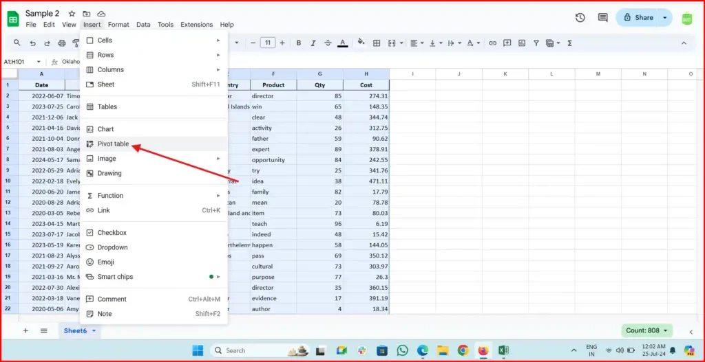
Open the Pivot Table Menu: Click on
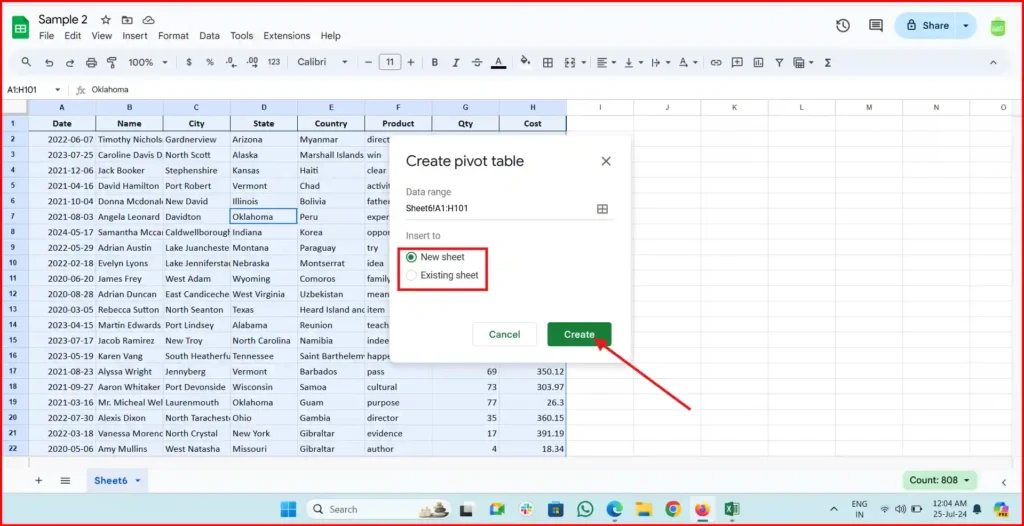
Insertin the top menu, then selectPivot tablefrom the dropdown list. You will be prompted to choose where you want to place your pivot table (either in a new sheet or an existing one).
how to sort date in pivot table by month Create the Pivot Table: Click
Createto generate a new pivot table.
how to sort months in pivot table google sheets
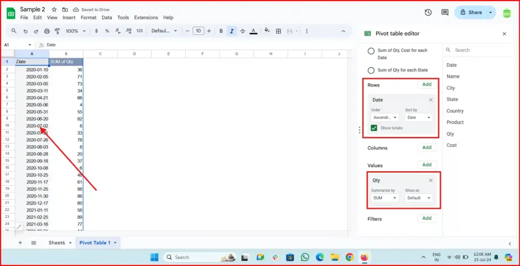
Step 3: Add Dates to the Pivot Table
Access Pivot Table Editor: On the right side of the screen, the Pivot table editor will appear.
Drag Date to Rows: In the Pivot table editor, you will see options to add rows, columns, values, and filters. Drag the date field into the
Rowsarea.
how to sort months in pivot table google sheets
Step 4: Group Dates by Month
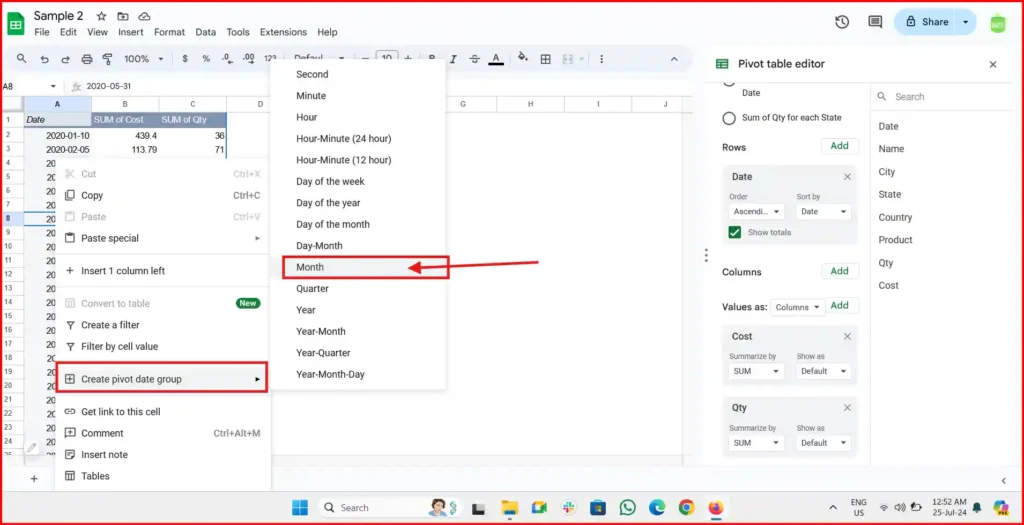
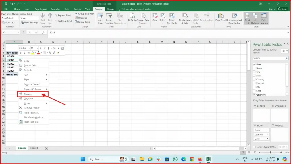
Right-Click on a Date: In the pivot table, right-click on any date within the date column.
note: Cursor must on the pivot dateshow to display months in ascending order in pivot table Group Dates: A menu will appear with options like
Year,Month,Week, etc. SelectMonth. This action will group the dates by month, and your pivot table will now display data aggregated by month.
how to show month wise in pivot table
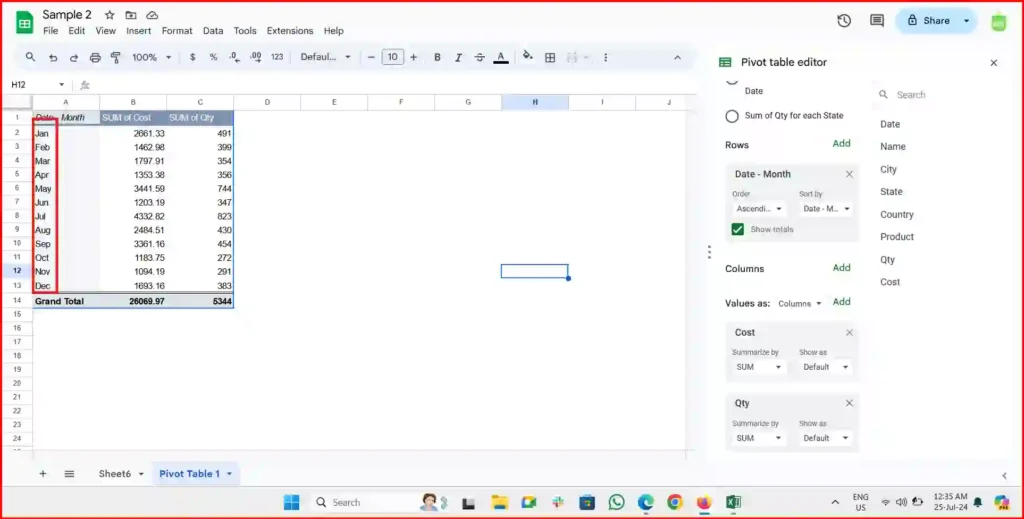
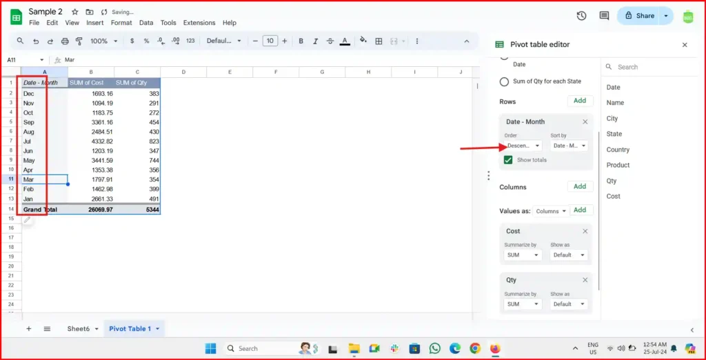
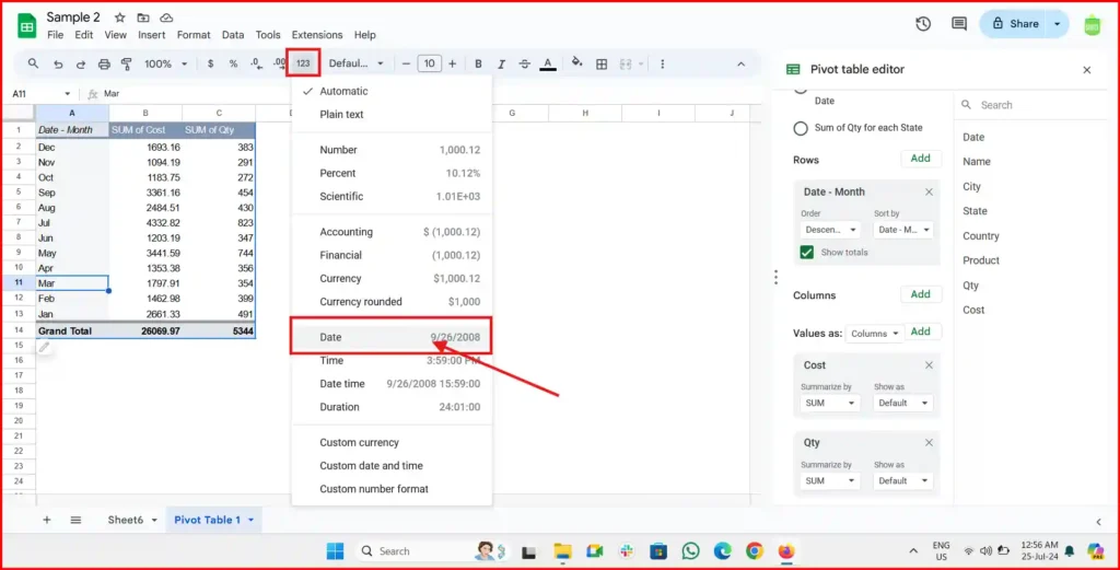
Step 5: Adjust the Order of Months
Sort Data: To change the order of the months, go back to the Pivot table editor. Click on the date field you dragged into the
Rowsarea.
how to sort months in pivot table google sheets Change Order: You will see options to sort the dates in ascending or descending order. Choose your preferred sorting option. Ascending order will display months from January to December, while descending order will display them from December to January.

how to group dates by month in pivot table in google sheets
Step 6: Verify Data Format( Optional in case group option not visible due invalid date)
Ensure that your dates are in a valid date format before creating the pivot table. If your dates are not recognized as dates by Google Sheets, you might need to reformat them. To do this:
Select Date Column: Highlight the column with dates.
Format as Date: Click on
Formatin the top menu, then selectNumberand chooseDate. This will ensure that Google Sheets recognizes your data as dates.
google sheets group by month and year
How to Show Months in Order in a Pivot Table in Excel
Pivot tables in Excel are a powerful tool for summarizing and analyzing large datasets. If your data includes dates and you want to group and order them by month, follow these simple steps to achieve that.
Step 1: Open Your Excel Workbook
Start by opening the Excel workbook that contains your data. Ensure your data includes a column with dates in a valid date format. If the dates are not formatted correctly, Excel might not group them as expected.
Step 2: Create a Pivot Table
To create a pivot table:
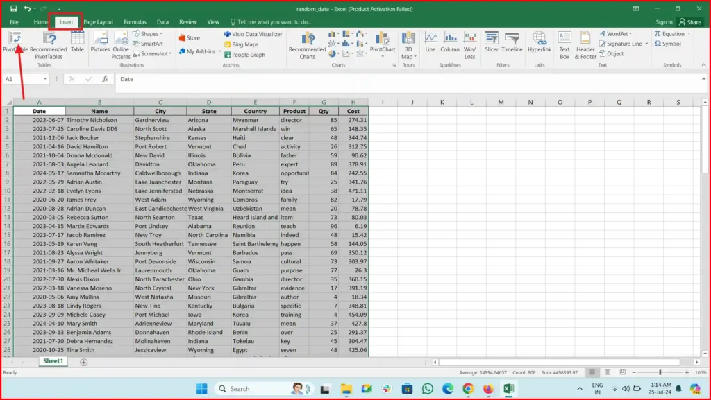
Select Your Data Range: Highlight the range of data you want to include in the pivot table. This should include your date column and any other relevant data.
Insert a Pivot Table: Go to the
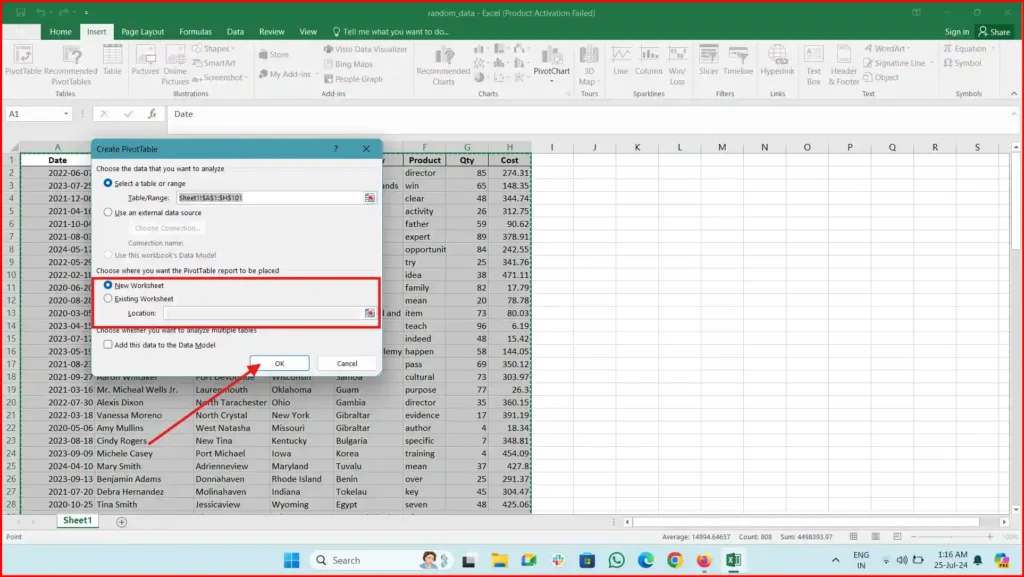
Inserttab in the top menu and click onPivotTable. You will be prompted to select the data range and choose where to place your pivot table (either in a new worksheet or an existing one).
How to arrange months in order in a pivot table Confirm the Pivot Table: Click
OKto create the pivot table.How do I sort months chronologically in a pivot table?
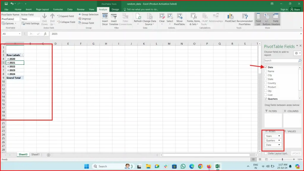
Step 3: Add Dates to the Pivot Table
Access PivotTable Fields: On the right side of the screen, the PivotTable Fields pane will appear.
Drag Date to Rows: Drag the date field into the
Rowsarea of the PivotTable Fields pane. Your pivot table will now display the dates in its rows.
pivot table date showing as year, quarter, month
Step 4: Group Dates by Month
Right-Click on a Date: In the pivot table, right-click on any date in the row labels.
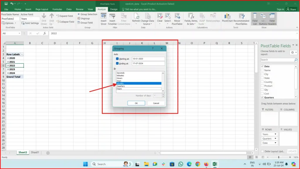
excel pivot table group dates by month and year Group Dates: From the context menu that appears, select
Group.... A dialog box will open with options to group byYears,Quarters,Months, etc. SelectMonths. You can also selectYearsif you want to group data within years.Click OK: After selecting
Months, clickOK. The dates in your pivot table will now be grouped by month.how to get month in order in pivot table
Step 5: Adjust the Order of Months
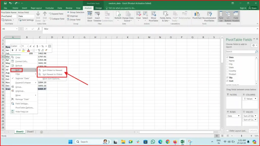
Sort Data: To change the order of the months, click on any month label in the pivot table.
ascending months in pivot table excel Sort Ascending or Descending: Go to the
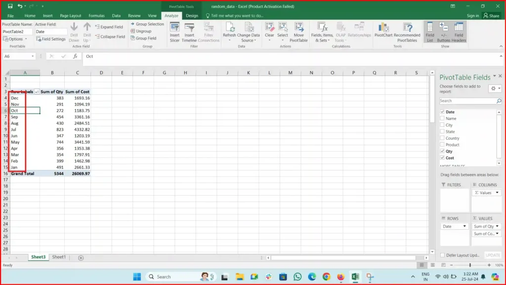
Datatab in the top menu, and use theSort AscendingorSort Descendingbuttons to order the months as desired. Ascending order will list the months from January to December, while descending will list them from December to January.how to sort in descending order in pivot table
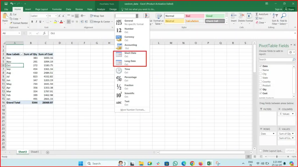
Step 6: Verify and Format Dates ( Optional in case group option not visible due invalid date)
Ensure your dates are formatted correctly:
Select Date Column: Highlight the column with dates in your original dataset.
Format as Date: Right-click on the selected column, choose
Format Cells, then selectDatefrom the category list. This ensures that Excel recognizes and processes your data as dates.
how to convert number to date in excel