How to find the last transaction date in Excel  let first know about excel and google Sheets, It is a versatile and powerful software for managing and analyzing data. Among the numerous tasks you can perform with it, finding the most recent transaction date for a list of products is a common requirement. This guide will walk you through the process step by step, ensuring you can easily fetch the most recent transaction dates for your products.

Want to learn how to merge multiple csv files in to one

Understanding the Data Structure

In your Google Sheets file named “sample,” you have two sheets:

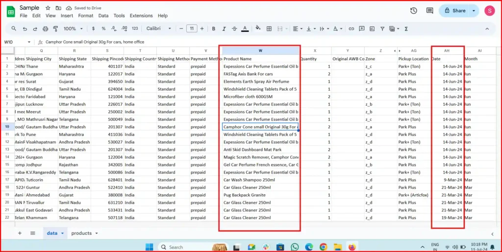
• Data: This sheet contains detailed transaction information.
  • • Date Column (AH): This column holds the dates of the transactions.
  • • Product Column (W): This column contains the names of the products involved in the transactions.

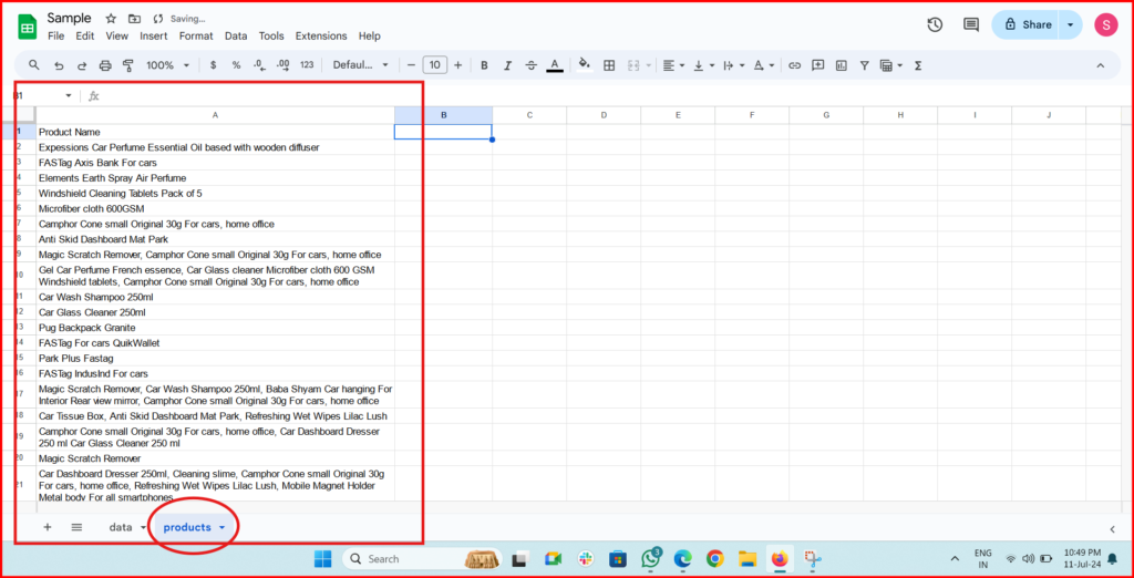
• Products Sheet: This sheet lists the products and is where you want to display the most recent transaction date for each product.

• • Product Names (A): This column contains the names of the products.

• • Last Transaction Date (B): This column will be used to display the most recent transaction date for each product.

Step-by-Step Guide to Finding the Most Recent Transaction Date

Step 1: Open Your Google Sheets File

How to find the last transaction date in Excel?

First, open your Google Sheets file named “sample.” Ensure that you have two sheets within this file: one named “data” and another named “products.”

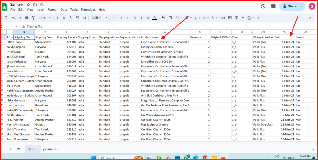
Step 2: Identify the Relevant Columns

In the “data” sheet, identify the columns that contain the relevant information:

• • Date: Located in column AH.

• • Product: Located in column W.

In the “products” sheet, identify the columns where the product names and last transaction dates will be:

• • Product Names: Located in column A.

• • Last Transaction Date: Located in column B.

Step 3: Enter the Formula

To fetch the most recent transaction date for each product, you will use the following formula in the “products” sheet:

=MAX(FILTER(data!AH:AH, data!W:W = A2))

Here’s how to enter the formula:

1. 1. Go to the “products” sheet.

1. 1. Click on cell B2 (the first cell in the Last Transaction Date column).

1. 1. Enter the formula: =MAX(FILTER(data!AH:AH, data!W:W = A2)).

Step 4: Understand the Formula

Let’s break down what this formula does:

• • FILTER(data!AH, data!W= A2):
    • • This part of the formula filters the dates in the “data” sheet (column AH) based on the product in column W that matches the product in A2 of the “products” sheet. Essentially, it finds all the dates for transactions involving the product listed in A2.

• • MAX():
    • • The MAX function then takes these filtered dates and returns the most recent one (the maximum date).

        
        how the formula will work watch this video GIF
        

How to find the last transaction date in Excel?

Step 5: Apply the Formula to All Products

Once you have entered the formula in cell B2, you need to apply it to all the products in your list. Here’s how to do it:

1. 1. Select cell B2.

1. 1. Click and drag the small square at the bottom-right corner of the cell down to copy the formula to the other cells in column B. This will apply the formula to all the products in column A.

Step 6: Verify the Results

After applying the formula to  all the products, double-check the “products” sheet to ensure that the last transaction dates are correctly displayed next to each product. Verify that the dates make sense and match the data in the “data” sheet.

Advanced Tips and Troubleshooting

While the basic formula works well for most cases, there are some advanced tips and common issues you might encounter: How to find the last transaction date in Excel

Using ArrayFormula for Improved Performance

If you have a large number of products, using the ArrayFormula function can improve performance. Here’s how to do it:

=ArrayFormula(IF(A2:A = "", "", MAX(FILTER(data!AH:AH, data!W:W = A2:A))))

This formula automatically applies to the entire column, which can be more efficient for larger datasets.

Ensuring Consistent Date Formats

To avoid errors, ensure that all dates in column AH of the “data” sheet are in the same format. Google Sheets can sometimes misinterpret dates if they are not consistently formatted, leading to incorrect results.

Handling Empty Cells

If you have empty cells in your product list, the formula might return an error. To handle this, you can modify the formula to check for empty cells:

=IF(A2 = "", "", MAX(FILTER(data!AH:AH, data!W:W = A2)))

This modification ensures that the formula only runs if there is a product name in column A.

Cross-Sheet References

Ensure that your references to other sheets (e.g., data!AH:AH) are correct. If you rename your sheets or move columns around, you will need to update the references in your formulas accordingly.

Practical Example

Let’s walk through a practical example to solidify your understanding:

Example Data

Imagine you have the following data in your “data” sheet.

And in your “products” sheet, you have the following list:

Applying the Formula

1. In cell B2 of the “products” sheet, enter the formula:

1. 1. In cell B2 of the “products” sheet, enter the formula:
      =MAX(FILTER(data!AH:AH, data!W:W = A2))

1. 1. Drag the formula down to cells B3 and B4.

Expected Results

The “products” sheet should now look like this:

This shows the most recent transaction dates for each product.

Benefits of This Method

Using this method to find the most recent transaction date offers several benefits:

Efficiency

Once set up, this method automatically updates the most recent transaction dates as new data is added to the “data” sheet. This saves time and reduces the risk of errors from manual updates.

Scalability

The formula can handle large datasets and many products, making it suitable for businesses of all sizes.

Accuracy

By using the MAX and FILTER functions, you ensure that the most recent date is always accurately retrieved from your data.

Conclusion

Finding the most recent transaction date for a list of products in Google Sheets is a straightforward process with the right formula. By following this step-by-step guide, you can efficiently manage your data and ensure accurate records.

Whether you are managing inventory, tracking sales, or analyzing trends, knowing the most recent transaction dates for your products is crucial. With this method, you can keep your data up-to-date and make informed decisions based on the latest information.

Feel free to experiment with the formulas and adjust them to fit your specific needs. Google Sheets offers a powerful platform for data management, and mastering these techniques will enhance your ability to analyze and utilize your data effectively.

Happy data analyzing!